5.1.2 Joint Cumulative Distributive Function (CDF)
Remember that, for a random variable $X$, we define the CDF as $F_X(x)=P(X \leq x)$. Now, if we have two random variables $X$ and $Y$ and we would like to study them jointly, we can define the joint cumulative function as follows:
The joint cumulative distribution function of two random variables $X$ and $Y$ is defined as
\begin{align}%\label{}
\nonumber F_{XY}(x,y)=P(X \leq x, Y \leq y).
\end{align}
As usual, comma means "and," so we can write
\begin{align}%\label{}
\nonumber F_{XY}(x,y)&=P(X \leq x, Y \leq y) \\
\nonumber &= P\big((X \leq x)\textrm{ and }(Y\leq y)\big)=P\big((X \leq x)\cap(Y\leq y)\big).
\end{align}
Figure 5.2 shows the region associated with $F_{XY}(x,y)$ in the two-dimensional plane. Note that the above definition of joint CDF is a general definition and is applicable to discrete, continuous, and mixed random variables.
Since the joint CDF refers to the probability of an event, we must have $0 \leq F_{XY}(x,y) \leq 1$.
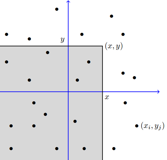
Figure 5.2: $F_{XY}(x,y)$ is the probability that $(X,Y)$ belongs to the shaded region. The dots are the pairs $(x_i,y_j)$ in $R_{XY}$.
If we know the joint CDF of $X$ and $Y$, we can find the marginal CDFs, $F_X(x)$ and $F_Y(y)$. Specifically, for any $x \in \mathbb{R}$, we have \begin{align}%\label{} \nonumber F_{XY}(x,\infty)&=P(X \leq x, Y \leq \infty) \\ \nonumber &= P(X \leq x)=F_X(x). \end{align} Here, by $F_{XY}(x,\infty)$, we mean $\lim \limits_{y \rightarrow \infty} F_{XY}(x,y)$. Similarly, for any $y \in \mathbb{R}$, we have \begin{align}%\label{} \nonumber F_Y(y)=F_{XY}(\infty, y). \end{align}Marginal CDFs of $X$ and $Y$:
\begin{align}\label{Eq:CDF-marginals} \nonumber F_X(x)&=F_{XY}(x, \infty)=\lim_{y \rightarrow \infty} F_{XY}(x,y), \hspace{20pt} \textrm{ for any } x,\\ F_Y(y)&=F_{XY}(\infty, y)=\lim_{x \rightarrow \infty} F_{XY}(x,y), \hspace{20pt} \textrm{ for any } y \hspace{20pt} (5.2) \end{align}Example
Let $X \sim Bernoulli(p)$ and $Y \sim Bernoulli(q)$ be independent, where $0<p,q<1$. Find the joint PMF and joint CDF for $X$ and $Y$.
- Solution
-
First note that the joint range of $X$ and $Y$ is given by
\begin{align}%\label{}
\nonumber R_{XY}=\{(0,0),(0,1),(1,0),(1,1)\}.
\end{align}
Since $X$ and $Y$ are independent, we have
\begin{align}%\label{}
\nonumber P_{XY}(i,j)=P_X(i)P_Y(j), \hspace{20pt} \textrm{for }i,j=0,1.
\end{align}
Thus, we conclude
\begin{align}%\label{}
\nonumber &P_{XY}(0,0)=P_X(0)P_Y(0)=(1-p)(1-q),\\
\nonumber &P_{XY}(0,1)=P_X(0)P_Y(1)=(1-p)q,\\
\nonumber &P_{XY}(1,0)=P_X(1)P_Y(0)=p(1-q),\\
\nonumber &P_{XY}(1,1)=P_X(1)P_Y(1)=pq.
\end{align}
Now that we have the joint PMF, we can find the joint CDF
\begin{align}
\nonumber F_{XY}(x,y)=P(X \leq x, Y \leq y).
\end{align}
Specifically, since $0 \leq X,Y \leq 1$, we conclude
\begin{align}
\nonumber &F_{XY}(x,y)=0, \hspace{20pt} \textrm{if } x<0,\\
\nonumber &F_{XY}(x,y)=0, \hspace{20pt} \textrm{if } y<0,\\
\nonumber &F_{XY}(x,y)=1, \hspace{20pt} \textrm{if } x \geq 1 \textrm{ and } y \geq 1.
\end{align}
Now, for $0 \leq x <1$ and $y \geq 1$, we have
\begin{align}%\label{}
\nonumber F_{XY}(x,y) &=P(X \leq x, Y \leq y)\\
\nonumber &= P(X=0, y \leq 1)\\
\nonumber &=P(X=0)=1-p.
\end{align}
Similarly, for $0 \leq y <1$ and $x \geq 1$, we have
\begin{align}%\label{}
\nonumber F_{XY}(x,y) &=P(X \leq x, Y \leq y)\\
\nonumber &= P(X \leq 1, y=0)\\
\nonumber &=P(Y=0)=1-q.
\end{align}
Finally, for $0 \leq x <1$ and $0 \leq y < 1$, we have
\begin{align}
\nonumber F_{XY}(x,y) &=P(X \leq x, Y \leq y)\\
\nonumber &= P(X=0, y=0)\\
\nonumber &=P(X=0)P(Y=0)=(1-p)(1-q).
\end{align}
Figure 5.3 shows the values of $F_{XY}(x,y)$ in different regions of the two-dimensional plane. Note that, in general, we actually need a three-dimensional graph to show a joint CDF of two random variables, i.e., we need three axes: $x$, $y$, and $z=F_{XY}(x,y)$. However, because the random variables of this example are simple, and can take only two values, a two-dimensional figure suffices.

Figure 5.3 Joint CDF for $X$ and $Y$ in Example 5.2
-
First note that the joint range of $X$ and $Y$ is given by
\begin{align}%\label{}
\nonumber R_{XY}=\{(0,0),(0,1),(1,0),(1,1)\}.
\end{align}
Since $X$ and $Y$ are independent, we have
\begin{align}%\label{}
\nonumber P_{XY}(i,j)=P_X(i)P_Y(j), \hspace{20pt} \textrm{for }i,j=0,1.
\end{align}
Thus, we conclude
\begin{align}%\label{}
\nonumber &P_{XY}(0,0)=P_X(0)P_Y(0)=(1-p)(1-q),\\
\nonumber &P_{XY}(0,1)=P_X(0)P_Y(1)=(1-p)q,\\
\nonumber &P_{XY}(1,0)=P_X(1)P_Y(0)=p(1-q),\\
\nonumber &P_{XY}(1,1)=P_X(1)P_Y(1)=pq.
\end{align}
Now that we have the joint PMF, we can find the joint CDF
\begin{align}
\nonumber F_{XY}(x,y)=P(X \leq x, Y \leq y).
\end{align}
Specifically, since $0 \leq X,Y \leq 1$, we conclude
\begin{align}
\nonumber &F_{XY}(x,y)=0, \hspace{20pt} \textrm{if } x<0,\\
\nonumber &F_{XY}(x,y)=0, \hspace{20pt} \textrm{if } y<0,\\
\nonumber &F_{XY}(x,y)=1, \hspace{20pt} \textrm{if } x \geq 1 \textrm{ and } y \geq 1.
\end{align}
Now, for $0 \leq x <1$ and $y \geq 1$, we have
\begin{align}%\label{}
\nonumber F_{XY}(x,y) &=P(X \leq x, Y \leq y)\\
\nonumber &= P(X=0, y \leq 1)\\
\nonumber &=P(X=0)=1-p.
\end{align}
Similarly, for $0 \leq y <1$ and $x \geq 1$, we have
\begin{align}%\label{}
\nonumber F_{XY}(x,y) &=P(X \leq x, Y \leq y)\\
\nonumber &= P(X \leq 1, y=0)\\
\nonumber &=P(Y=0)=1-q.
\end{align}
Finally, for $0 \leq x <1$ and $0 \leq y < 1$, we have
\begin{align}
\nonumber F_{XY}(x,y) &=P(X \leq x, Y \leq y)\\
\nonumber &= P(X=0, y=0)\\
\nonumber &=P(X=0)P(Y=0)=(1-p)(1-q).
\end{align}
Figure 5.3 shows the values of $F_{XY}(x,y)$ in different regions of the two-dimensional plane. Note that, in general, we actually need a three-dimensional graph to show a joint CDF of two random variables, i.e., we need three axes: $x$, $y$, and $z=F_{XY}(x,y)$. However, because the random variables of this example are simple, and can take only two values, a two-dimensional figure suffices.
Here is a useful lemma:
LemmaFor two random variables $X$ and $Y$, and real numbers $x_1 \leq x_2$, $y_1 \leq y_2$, we have \begin{align}%\label{} \nonumber P(x_1<X &\leq x_2, \hspace{5pt} y_1<Y \leq y_2)= \\ \nonumber &F_{XY}(x_2,y_2)-F_{XY}(x_1,y_2)-F_{XY}(x_2,y_1)+F_{XY}(x_1,y_1). \end{align} To see why the above formula is true, you can look at the region associated with $F_{XY}(x,y)$ (as shown in Figure 5.2) for each of the pairs $(x_2,y_2), (x_1,y_2), (x_2,y_1), (x_1,y_1)$. You can see, as we subtract and add regions, the part that is left is the region $\{x_1<X \leq x_2, \hspace{5pt} y_1<Y \leq y_2\}$.

