---

In this section, we will use the Dirac delta function to analyze mixed random variables. Technically speaking, the Dirac delta function is not actually a function. It is what we may call a generalized function. Nevertheless, its definition is intuitive and it simplifies dealing with probability distributions.

Remember that any random variable has a CDF. Thus, we can use the CDF to answer questions regarding discrete, continuous, and mixed random variables. On the other hand, the PDF is defined only for continuous random variables, while the PMF is defined only for discrete random variables. Using delta functions will allow us to define the PDF for discrete and mixed random variables. Thus, it allows us to unify the theory of discrete, continuous, and mixed random variables.

Dirac Delta Function

Remember, we cannot define the PDF for a discrete random variable because its CDF has jumps. If we could somehow differentiate the CDF at jump points, we would be able to define the PDF for discrete random variables as well. This is the idea behind our effort in this section. Here, we will introduce the Dirac delta function and discuss its application to probability distributions. If you are less interested in the derivations, you may directly jump to Definition 4.3 and continue from there. Consider the unit step function $u(x)$ defined by \begin{equation} \hspace{50pt} u(x) = \left\{ \begin{array}{l l} 1 & \quad x \geq 0 \\ 0 & \quad \text{otherwise} \end{array} \right. \hspace{50pt} (4.8) \end{equation} This function has a jump at $x=0$. Let us remove the jump and define, for any $\alpha > 0$, the function $u_{\alpha}$ as \begin{equation} \nonumber u_{\alpha}(x) = \left\{ \begin{array}{l l} 1 & \quad x > \frac{\alpha}{2} \\ \frac{1}{\alpha} (x+\frac{\alpha}{2}) & \quad -\frac{\alpha}{2} \leq x \leq \frac{\alpha}{2} \\ 0 & \quad x < -\frac{\alpha}{2} \end{array} \right. \end{equation} The good thing about $u_{\alpha}(x)$ is that it is a continuous function. Now let us define the function $\delta_{\alpha}(x)$ as the derivative of $u_{\alpha}(x)$ wherever it exists. \begin{equation} \nonumber \delta_{\alpha}(x)=\frac{ d u_{\alpha}(x)}{dx} = \left\{ \begin{array}{l l} \frac{1}{\alpha} & \quad |x| < \frac{\alpha}{2} \\ 0 & \quad |x| > \frac{\alpha}{2} \end{array} \right. \end{equation} Figure 4.10 shows these functions.

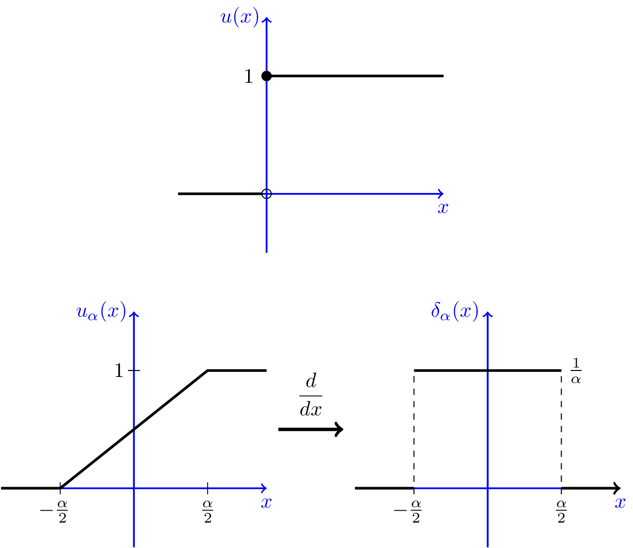
We notice the following relations: $$\hspace{50pt} \delta_{\alpha}(x)=\frac{d}{dx} u_{\alpha}(x), \hspace{15pt} u(x) \overset{\text{a.e.}}{=} \lim_{\alpha \rightarrow 0} u_{\alpha}(x) \hspace{50pt} (4.9)$$ Now, we would like to define the delta "function", $\delta(x)$, as $$\hspace{100pt} \delta(x)=\lim_{\alpha \rightarrow 0} \delta_{\alpha}(x) \hspace{100pt} (4.10)$$ Note that as $\alpha$ becomes smaller and smaller, the height of $\delta_{\alpha}(x)$ becomes larger and larger and its width becomes smaller and smaller. Taking the limit, we obtain \begin{equation} \nonumber \delta(x) = \left\{ \begin{array}{l l} \infty & \quad x=0 \\ 0 & \quad \text{otherwise} \end{array} \right. \end{equation} Combining Equations 4.9 and 4.10, we would like to symbolically write $$\delta(x)=\frac{d}{dx} u(x).$$ Intuitively, when we are using the delta function, we have in mind $\delta_{\alpha}(x)$ with extremely small $\alpha$. In particular, we would like to have the following definitions. Let $g:\mathbb{R} \mapsto \mathbb{R}$ be a continuous function. We define $$\hspace{50pt} \int_{-\infty}^{\infty} g(x) \delta(x-x_0) dx = \lim_{\alpha \rightarrow 0} \bigg[ \int_{-\infty}^{\infty} g(x) \delta_{\alpha} (x-x_0) dx \bigg] \hspace{50pt} (4.11)$$ Then, we have the following lemma, which in fact is the most useful property of the delta function.

Lemma

Let $g:\mathbb{R} \mapsto \mathbb{R}$ be a continuous function. We have $$\int_{-\infty}^{\infty} g(x) \delta(x-x_0) dx = g(x_0).$$

Proof

Let $I$ be the value of the above integral. Then, we have

$I$	$= \lim_{\alpha \rightarrow 0} \bigg[ \int_{-\infty}^{\infty} g(x) \delta_{\alpha} (x-x_0) dx \bigg]$
	$=\lim_{\alpha \rightarrow 0} \bigg[ \int_{x_0-\frac{\alpha}{2}}^{x_0+\frac{\alpha}{2}} \frac{g(x)}{\alpha} dx \bigg].$

By the mean value theorem in calculus, for any $\alpha>0$, we have $$\int_{x_0-\frac{\alpha}{2}}^{x_0+\frac{\alpha}{2}} \frac{g(x)}{\alpha} dx=\alpha \frac{g(x_{\alpha})}{\alpha}=g(x_{\alpha}),$$ for some $x_{\alpha} \in (x_0-\frac{\alpha}{2},x_0+\frac{\alpha}{2}).$ Thus, we have $$I = \lim_{\alpha \rightarrow 0} g(x_{\alpha})=g(x_0).$$ The last equality holds because $g(x)$ is a continuous function and $\lim_{\alpha \rightarrow 0} x_{\alpha}=x_0$.

For example, if we let $g(x)=1$ for all $x \in \mathbb{R}$, we obtain $$\int_{-\infty}^{\infty} \delta(x) dx =1.$$ It is worth noting that the Dirac $\delta$ function is not strictly speaking a valid function. The reason is that there is no function that can satisfy both of the conditions $$\delta(x)=0 (\textrm{ for }x \neq 0) \hspace{20pt} \textrm{and} \hspace{20pt} \int_{-\infty}^{\infty} \delta(x) dx =1.$$ We can think of the delta function as a convenient notation for the integration condition 4.11. The delta function can also be developed formally as a generalized function. Now, let us summarize properties of the delta function.

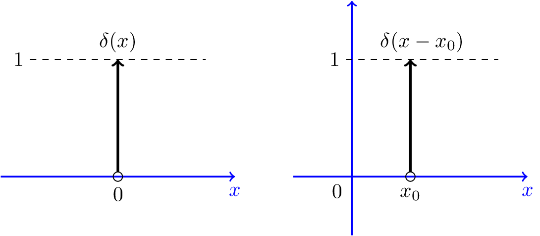
Figure 4.11 shows how we represent the delta function. The delta function, $\delta(x)$, is shown by an arrow at $x=0$. The height of the arrow is equal to $1$. If we want to represent $2\delta(x)$, the height would be equal to $2$. In the figure, we also show the function $\delta(x-x_0)$, which is the shifted version of $\delta(x)$.

Using the Delta Function in PDFs of Discrete and Mixed Random Variables

In this section, we will use the delta function to extend the definition of the PDF to discrete and mixed random variables. Consider a discrete random variable $X$ with range $R_X=\{x_1,x_2,x_3,...\}$ and PMF $P_X(x_k)$. Note that the CDF for $X$ can be written as $$F_X(x)=\sum_{x_k \in R_X} P_X(x_k)u(x-x_k).$$ Now that we have symbolically defined the derivative of the step function as the delta function, we can write a PDF for $X$ by "differentiating" the CDF:

$f_X(x)$	$=\frac{dF_X(x)}{dx}$
	$=\sum_{x_k \in R_X} P_X(x_k)\frac{d}{dx} u(x-x_k)$
	$=\sum_{x_k \in R_X} P_X(x_k)\delta(x-x_k).$

We call this the generalized PDF.

Note that for any $x_k \in R_X$, the probability of $X=x_k$ is given by the coefficient of the corresponding $\delta$ function, $\delta(x-x_k)$.

It is useful to use the generalized PDF because all random variables have a generalized PDF, so we can use the same formulas for discrete, continuous, and mixed random variables. If the (generalized) PDF of a random variable can be written as the sum of delta functions, then $X$ is a discrete random variable. If the PDF does not include any delta functions, then $X$ is a continuous random variable. Finally, if the PDF has both delta functions and non-delta functions, then $X$ is a mixed random variable. Nevertheless, the formulas for probabilities, expectation and variance are the same for all kinds of random variables.

To see how this works, we will consider the calculation of the expected value of a discrete random variable. Remember that the expected value of a continuous random variable is given by $$EX=\int_{-\infty}^{\infty} xf_X(x)dx.$$ Now suppose that I have a discrete random variable $X$. We can write

$EX$	$=\int_{-\infty}^{\infty} xf_X(x)dx$
	$=\int_{-\infty}^{\infty} x\sum_{x_k \in R_X} P_X(x_k)\delta(x-x_k)dx$
	$=\sum_{x_k \in R_X} P_X(x_k) \int_{-\infty}^{\infty} x \delta(x-x_k)dx$
	$=\sum_{x_k \in R_X} x_kP_X(x_k)$	$\textrm{by the 4th property in Definition 4.3,}$

which is the same as our original definition of expected value for discrete random variables. Let us practice these concepts by looking at an example.

---

Example

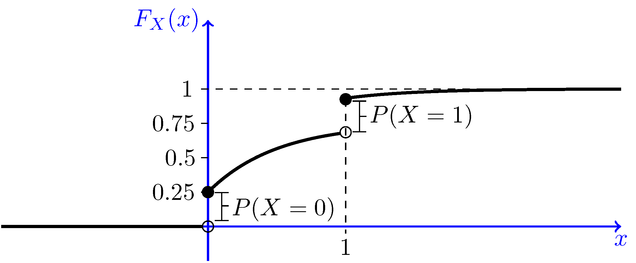
Let $X$ be a random variable with the following CDF: \begin{equation} \nonumber F_X(x) = \left\{ \begin{array}{l l} \frac{1}{2}+ \frac{1}{2}(1-e^{-x})& \quad x \geq 1\\ \frac{1}{4}+ \frac{1}{2}(1-e^{-x})& \quad 0 \leq x < 1\\ 0 & \quad x < 0 \end{array} \right. \end{equation}

1. What kind of random variable is $X$ (discrete, continuous, or mixed)?
2. Find the (generalized) PDF of $X$.
3. Find $P(X>0.5)$, both using the CDF and using the PDF.
4. Find $EX$ and Var$(X)$.

---

In general, we can make the following statement:

---